Recently, I’ve been involved in experiment design and measurement - specifically AB Testing. This experience has encouraged me to learn more about experimentation because of unique challenges faced with conversion optimisation. This post, goes hand in hand with lead score experimentation.
In brief, the unique challenges posed were:
- Dealing with largely a non-technical audience
- Low sample sizes
- Costly human interventions as a variant.
Because of this, I chose Bayesian AB Testing as a measurement framework. In brief, without bashing Frequentist methods, some benefits of Bayesian AB testing are:
- Whilst not immune to peeking, you can analyse results during an experiment with caution. This was good keeping stakeholders engaged throughout the journey.
- There are no p-values, instead you get a Probability of X being better than Y. This is is a lot easier to explain to non-technical stakeholders.
- There is potential for faster experiments when compared to traditional AB testing.
Literature on Bayesian AB testing is readily available, so I won’t go into a lot of detail explaining how it works. A good guide is available here from Dynamic Yield.
A great quote from the above post that lays the foundation for this is post is:
“The math behind the Bayesian framework is quite complex so I will not get into it here. In fact, I would argue that the fact that the math is more complicated than can be computed with a simple calculator or Microsoft Excel is a dominant factor in the slow adoption of this method in the industry.”
Whilst Dynamic Yield also offers a great calculator here that you can use for your experiments. This post is designed to give you a light understanding of the math behind Bayesian AB testing and also how to code your own model in Python with Pyro.
Introducing Pyro
Pyro is a universal probabilistic programming language (PPL) written in Python and supported by PyTorch on the backend. It was originally open sourced by Uber AI.
It is a highly flexible language similar to PyMC3 and Stan, and whilst it’s uses and functionality far exceed AB testing - it is perfectly suited to this type of problem.
Let’s get started
To give an illustrative example, let’s assume your start-up is trialling methods of converting trialists. To assist in conversion you can either:
- Call the customer
- Email the customer
And you want to know what channel is performing better – calling or emailing?
We can summarise the results as below:
| Method | Attempts/Reach | Conversions |
|---|---|---|
| 700 | 73 | |
| Call | 200 | 35 |
Something to notice is our sample sizes are different between each campaign. This is an advantage that Bayesian AB testing can give you over Frequentist testing.
Defining the model
Since we’re measuring a Yes/No event, we should use the Binomial distribution to model conversion events. Now that we’ve specified the posterior distribution how do we influence the Binomial rate?
This is where the conjugate prior comes in, as the Beta distribution is the conjugate prior for the Binomial distribution - we’ll use the Beta distribution. In this model, we use a $Beta(2,2)$ prior, which effectively says our prior belief is that conversion is 50% and is equally likely to be higher or lower. Of course, once we condition this with actual data this belief will quickly adjust.
As an example, let’s say that we’ve already run an email campaign and it had a conversion rate of 20% and now we’re wanting to test to see if a costly campaign such as calling is more effective. As it would be a shame to waste the knowledge we already have, we could encode our knowledge with a prior such as $Beta(5, 20)$. This difference can be illustrated with the following graph.
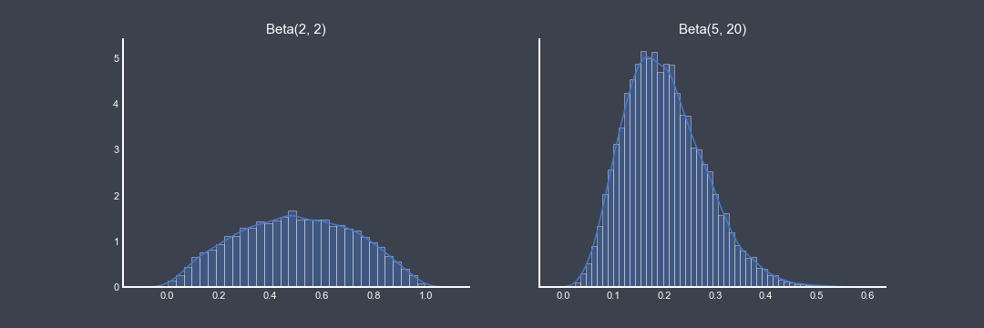
In terms of running an experiment, we have the potential to get faster results than a traditional AB test by using informative priors. As well as the continual updating nature of Bayesian testing, we can capture run-away winners (or losses) earlier than a fixed AB test.
In Pyro this model will look like:
import pyro
import pyro.distributions as dist

def ab_model(obs_call , obs_email, n_call, n_email):
    prior_call = pyro.sample("prior_call", dist.Beta(2., 2.))
    prior_email = pyro.sample("prior_email", dist.Beta(2., 2.))
    difference = pyro.deterministic("difference", prior_call - prior_email)

    with pyro.plate('likelihood', 1000):
        likelihood_call = pyro.sample("likelihood_call", dist.Binomial(total_count=n_call, probs=prior_call), obs=obs_call)
        likelihood_email= pyro.sample("likelihood_email", dist.Binomial(total_count=n_email, probs=prior_email), obs=obs_email)
If you’re familiar with Python, the first thing you’ll notice is that this looks like a regular function. This is definitely one of the strengths of Pyro.
To begin, prior_email and prior_call are where we define our Beta priors. This is an interesting point that’s worth further discussion.
The goal of this experiment is to test the differences between our two campaigns. Whilst this parameter isn’t necessary, it can be helpful to wrap the difference between prior_call - prior_email within the pyro.deterministic. Which returns a single point estimate (MAP).
Running the model
Before we run the model, it’s helpful to think of the data format our model can take. Both of these are valid:
obs_call = [1, 0, ...., 1, 1]
obs_call = 35
As you can see you can pass through a list of Binomial observations or single integer.
The next step is to condition or model on our observed data. Pyro has two main ways of doing this: Variational Inference, and Markov Chain Monte Carlo (MCMC) simulations. We’ll use MCMC as follows:
from pyro.infer.mcmc import NUTS, MCMC

nuts = NUTS(ab_model, adapt_step_size=True)

mcmc = MCMC(nuts, num_samples=3000, warmup_steps=200)

mcmc.run(
	torch.tensor(obs_v1, dtype=torch.double),
	torch.tensor(obs_v2, dtype=torch.double),
	torch.tensor(n_1, dtype=torch.double),
	torch.tensor(n_2, dtype=torch.double)
)
Interpreting Results
The most simple way to view the results, is by running mcmc.summary(). This will display the mean and standard deviations of prior_call and prior_email - representing the estimated conversion rates that these campaigns achieved.
How can we quantify the uncertainty of which campaign performed better? This is where Bayesian testing really shines. To get this, we can use the difference we defined in our model.
samples = Predictive(ab_model, num_samples=1000, return_sites=['difference'])

samples = samples.get_samples(
    torch.tensor(obs_v1, dtype=torch.double),
    torch.tensor(obs_v2, dtype=torch.double),
    torch.tensor(n_1, dtype=torch.double),
    torch.tensor(n_2, dtype=torch.double)
)

print(np.mean(samples['difference'].numpy() > 0))
This will return a probability of Calling being better than Emailing. Of course, this can be flipped around with a probability that Calling is not better than emailing.
Extending AB Testing
The most logical extension is for situations where we have multiple variants. Bayesian AB testing can extend nicely to this, without using the bonferroni correction.
Another extension would be to consider revenue and costs associated to campaigns. Bayesian AB testing is flexible enough to incorporate monetary effects, and because of the intuitive nature of Bayesian AB testing you can yield business insight.