Today, I will take you through a simple next-word prediction model built using PyTorch.
The inspiration for this, is of course predictive text - or more specifically Google’s Smart Compose. At its core, the Google Smart Compose model is a form of language model. Smart Compose uses a few words the user inputs and then predicts the following words or sentences in emails you want to write.

Google details how they build their Smart Compose feature in their research blog post here. From this, I want to pull out some requirements for building a successful Smart Compose model:
- Latency. Latency is important, it must generate a response in under 100ms.
- They explored a Sequence to sequence-style model (Seq2seq) but found it failed the latency test. Instead, they opted for a Recurrent neural network (RNN) model.
Therefore, let’s build a fast RNN based model to predict the next word! Now, I know that in the age of large language models such as GPT, LLaMA or Google’s on Gemma/Gemini models, these more simple applications are overlooked. However, the basis of this Smart Compose model helps us build the foundational understanding to grasp the technical details of transformers, and larger models.
Smaller, more simple models such as these can often outperform large language models and are naturally better suited for edge applications due to their smaller size.
Look into RNNs
Recurrent neural networks (RNN) are a class of neural network that allow for previous outputs to be used as inputs. As the sequence of inputs is passed through the model, the weights of previous inputs are also used as inputs.
This ability to remember previous inputs is akin to how we humans read. We read in a single direction (left to right, or right to left), and we recall what previous words have been used to understand the meaning of a sentence and then paragraph.
Traditional networks, such as feed-forward or convolutional networks, don’t have this ability to remember previous information. Once they scan a given input, they move on, forgetting all the previous inputs.
RNN’s ability to use previous inputs naturally makes RNN models well-suited for sequential data such as text, time series, audio, etc.
One type of RNN architecture is the LSTM. LSTM stands for Long Short-Term Memory. As the name suggests, LSTMs are capable of learning long-term dependencies. LSTMs are seen as an improvement over vanilla RNN layers due to them being designed to overcome vanishing gradient problem - a problem you may while training vanilla RNN.
Both, LSTM and Gated Recurrent Units (GRU, another variation on an RNN) have a more complex structure than an RNN, these comprise - comprising of three gates:
- Input gate
- Output gate
- Forget gate.
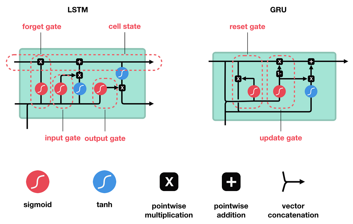
These three gates represent sigmoid layers, which control how much information can enter, leave or be forgotten within the layer.
The input gate plays a role in determining which information from the current input should be stored in the cell state. By selectively controlling the update of the LSTM cell state, it discerns the relevance of new input data.
In contrast, the forget gate serves to decide which information from the previous cell state should be retained or discarded. Selectively erasing outdated or irrelevant information ensures that the LSTM cell state remains focused on relevant tasks.
Finally, the output gate functions to regulate the information that is output from the LSTM cell state. By filtering the contents of the cell state, it determines the final output of the LSTM cell, considering both the current input and the memory stored within the cell state.
These three gates enable the LSTM cell to manage and process sequential data effectively. This is an extremely good post if you want a complete in-depth understanding of LSTM layers.
PyTorch Model
Let’s start now by introducing the model code, then explaining each part. For the brevity of this post, we’ll skip the data loading, tokenising and training of the model. However, the accompanying Google Colab notebook has this. I use PyTorch Lightning in the notebook to abstract away some of the boilerplate code needed.
class Model(nn.Module):
	def __init__(self,
		embedding_dim: int,
		hidden_dim: int,
		vocab_size: int,
		num_layers: int = 1
	):
		super(Model, self).__init__()

		self.hidden_dim = hidden_dim
		self.word_embeddings = nn.Embedding(vocab_size, embedding_dim)
		# The LSTM takes word embeddings as inputs, and outputs hidden states
		# with dimensionality hidden_dim.
		self.lstm = nn.LSTM(embedding_dim, hidden_dim, num_layers, batch_first=True)
		# The linear layer that maps from hidden state space to vocab size
		self.fc = nn.Linear(hidden_dim, vocab_size)

	def forward(self, sentence):
		embeds = self.word_embeddings(sentence)
		lstm_out, _ = self.lstm(embed)
		output = self.fc(lstm_out[:, -1, :])
		return output
In terms of models, this is quite a straight-forward one. With the following config, we get 65.4 million parameters:
model_config = {
	'embedding_dim': 128,
	'hidden_dim': 256,
	'num_layers': 2,
	'vocab_size': len(vocab) # is equal to XXXX
}
Embedding layer
Embeddings have come to the forefront with the rise of generative AI. The role embeddings play here is in compressing the potentially mammoth vocabulary size (vocab_size), down to a more manageable dimension of embed_size dimensions.
This embedding layer will help play a role within associated similar words close together within the embed_size vector space. You can read more about embeddings here.
LSTM Layers
The next layer is our LSTM layer; this is the PyTorch implementation of what we described above. It takes the output of our embedding layer (embed_size), and outputs a tensor with hidden_dim.
Linear Layer
This final layer is our fully connected linear layer. The input of size of this model is our hidden_dim from our LSTM layer, and the output size is our vocab_size.
Put another way, we are trying to predict the next word given our known vocab_size. This linear layer outputs logits, which we can then pass through into a softmax function to transform into probabilities.
Predicting the next word.
Finally, I want to get into the predict function. The code is presented below.
def predict(prompt: str, max_seq_len: int, temperature: float, model, tokenizer, vocab, device, seed=None):
	if seed is not None:
		torch.manual_seed(seed)

	model.eval()
	tokens = tokenizer(prompt)
	indices = [vocab[t] for t in tokens]
	batch_size = 1

	with torch.no_grad():
		for i in range(max_seq_len):
			src = torch.LongTensor([indices]).to(device)
			prediction = model(src)
			probs = torch.softmax(prediction[:, -1] / temperature, dim=-1)
			prediction = torch.multinomial(probs, num_samples=1).item()
			while prediction == vocab['<unk>']:
				prediction = torch.multinomial(probs, num_samples=1).item()

			if prediction == vocab['<eos>']:
				break
			indices.append(prediction)

		itos = vocab.get_itos()

		tokens = [itos[i] for i in indices]

		return tokens
In this function, we have a prompt; this could be the start of the sentence. We have a max_seq_len argument that limits the number of words generated. That is to say, this function will keep predicting the following words until max_seq_len is met or the model itself predicts <eos>, indicating that the text has finished.
We apply a temperature argument here. Temperature is a common parameter within generation models and works to ’temper’ the model’s confidence in the most likely predicted output. As temperature increases, this increases the probability that lower predicted tokens will be selected by the next line where we sample the Multinomial distribution. This blog has a brilliant visualisation of this.
Grounding the model with context
One way to improve the model would be to try to provide the model context as to what it’s predicting. For example, writing an email to a friend would be very different to writing an email enquiring about a job.
Our two resources on the Smart compose model come from the blog post mentioned above and the associated research paper, in which the paper goes into more detail.
Google attempts to do just this! They try to ground the model with context by embedding the Subject line and previous messages into the model and concatenating this embedding with the input to the model. The helps model predicts a relevant sentence given the context in which the email is being written.

You can re-create this by adding two separate embedding layers within your model and concatenating the outputs. The following pseudo-code represents this:
class Model(nn.Module):
	def __init__(self):
		super(Model, self).__init__()
		subject_embedding = nn.Embedding(subject_size, embedding_dim)
		prev_embedding = nn.Embedding(prev_size, embedding_dim)
		...

	def forward(self, batch):
		subject, prev, ... = batch
		emb_subject = self.subject_embedding(subject)
		emb_prev = self.prev_embedding(prev)

		cat = torch.cat(emb_subject, emb_prev)
		...
Applications
Prediction models can help predict what to say next, encouraging users to give more details on customer support issues for example.
They can also help guide customers to the right terms to search within e-commerce or job boards.
Ultimately, being comparatively lightweight to generative models, next word prediction can have much lower latency and much lower costs, while both increasing the customer experience and helping drive business metrics.